Occupancy Grid Maps

We have covered the Kalman Filter, the Extended Kalman Filter, and briefly mentioned alternatives. Now we move to particle filters — but before we do, we introduce grid maps, an alternative to the landmark/feature representation used by the KF approaches.

This lesson covers grid maps; the next lessons cover Monte Carlo localization, FastSLAM, and grid-based SLAM.

Feature-based vs occupancy-based mapping

• Feature/landmark-based SLAM needs a front-end that detects features from the sensor feed (camera, LiDAR, …).
• Occupancy maps can be derived directly from sensor measurements (typically LiDARs) with no additional processing.

Features / landmarks

• Natural choice for Kalman-Filter–based systems.
• Compact representation.
• Multiple observations of the same landmark improve its position estimate (EKF).
• Requires a reliable feature detector.

Grid maps

• Discretize the world into cells.
• Each cell is assumed to be occupied or free.
• Non-parametric model.
• Large maps require substantial memory.
• Do not rely on a feature detector.

Assumptions

Each cell $m_i$ is a binary random variable modelling occupancy:

• Occupied: $p(m_i)\to 1$
• Free: $p(m_i)\to 0$
• No knowledge: $p(m_i)=0.5$

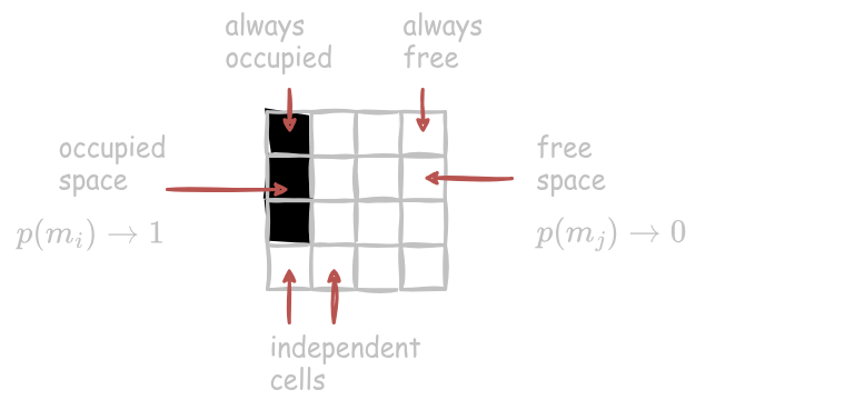
1. Binary cell state. The area corresponding to a cell is either completely free or occupied.
2. Static world. The world is static — cells don't change once observed.
3. Cell independence. Cells are independent random variables.

Note. Cell independence is a convenient approximation, not a faithful property of real environments. Occupancy is spatially correlated (a wall is a long surface), but assuming independence keeps updates factorized and online — one Bayes / log-odds update per cell.

Representation

The map distribution is the product over the cells:

Given sensor data $z_{1:t}$ and known poses $x_{1:t}$, we estimate:

where $m_i$ is a binary random variable. We use a Bayes filter per cell — simpler than the full Bayes filter because the world is static, so there is no prediction step.

↳ This is the binary Bayes filter for static state.

Static-state binary Bayes filter (derivation)

Start by applying Bayes' rule to the cell posterior:

Apply the Markov assumptions:

• Knowing where the robot will be in the future gives no extra information about a current cell: $p(m_i\mid z_{1:t-1},x_{1:t})\to p(m_i\mid z_{1:t-1},x_{1:t-1})$
• Given the cell state, past observations don't help predict the current one: $p(z_t\mid m_i,z_{1:t-1},x_{1:t})\to p(z_t\mid m_i,x_{1:t})$

Eq. (1) becomes:

Now flip the likelihood by applying Bayes' rule again:

Substitute (3) into (2), and assume that without an observation the pose $x_t$ alone tells us nothing about the cell — $p(m_i\mid x_t)\to p(m_i)$:

Doing the same thing for $\neg m_i$ (cell is free) gives a symmetric expression. Dividing the two cancels the messy normalizers $p(z_t\mid x_t)$ and $p(z_t\mid z_{1:t-1},x_{1:t})$:

Three clean factors — a fresh-measurement term, a recursive term, and a prior. We can invert the ratio to recover the probability:

In practice we run the update in log-odds — products turn into sums, no exponentials.

Log-odds notation

Define the log-odds:

Recover the probability via $p(x)=1-\frac{1}{1+\exp \ell (x)}$.

The occupancy update becomes additive:

Or in shorthand:

Occupancy grid mapping algorithm

Inverse sensor model (laser range finder)

The inverse sensor model turns a single LiDAR beam into per-cell occupancy evidence. It supplies the $p(m_i=1\mid z_t,x_t)$ term needed by the log-odds update, converting one ray into many local map updates.

Inputs (per beam): measured range $z$, beam direction, grid geometry. Outputs (per touched cell): a probability (or log-odds increment) that the cell is occupied.

Physical encoding:

• Free before the hit. Cells with distance $s<z-\frac{r}{2}$ are pushed toward free with probability $p_{\text{free}}$.
• Hit window. Cells in the thin window $[z-\frac{r}{2},z+\frac{r}{2}]$ are marked occupied with probability $p_{\text{occ}}$.
• Beyond the hit. For $s>z+\frac{r}{2}$ we provide no information and keep the prior $p_{\text{prior}}$.

The window width $r$ (typically 1–3 cell widths) absorbs range/bearing noise and grid discretization so observed surfaces leave a stable, thin footprint.

Piecewise definition (per cell at distance $s$ along the ray):

• Max-range case. If the beam returns no hit, apply free-space evidence up to $z$; beyond $z$ keep the prior.
• Independence. Each touched cell is updated independently; ray-casting decides which cells are touched. Convert probabilities to log-odds increments with $\Delta \ell =\log \frac{p}{1-p}-{\ell }_0$, then apply the standard update.

import numpy as np
 
def p_occ_step(s_i, z, r, p_free, p_prior, p_occ):
    """Inverse sensor model with a step window."""
    left  = z - r / 2.0
    right = z + r / 2.0
    if s_i < left:
        return p_free
    elif s_i <= right:
        return p_occ
    else:
        return p_prior

Drag the sliders to see how the inverse sensor model's piecewise profile depends on the measured range and the window width. Cells inside the hit window are pushed toward p_occ; cells before it are pushed toward p_free; cells beyond the hit stay at the prior 0.5.

This interactive map shows the algorithm running: the rotating LiDAR beam on the left builds up the log-odds occupancy map on the right via the inverse-sensor-model update. As the robot walks around (or you click to teleport it), more cells get pushed toward 0 (free, white) or 1 (occupied, black); unobserved cells stay at the prior grey.

Summary

• Occupancy grid maps discretize space into independent cells.
• Each cell is a binary random variable estimating whether the cell is occupied.
• We run a static-state binary Bayes filter per cell.
• Mapping with known poses is easy.
• The log-odds representation makes the update additive and fast.
• No need for pre-defined features.

Incremental scan alignment (bonus)

Trying to make an occupancy map from raw odometry doesn't work well in practice.

• Motion is noisy; we can't ignore it.
• Assuming known poses fails.
• Often the sensor is more precise than the odometry.
• Scan matching incrementally aligns two scans, or a scan to a map, without revisiting the past.

Pose correction via scan matching (MAP):

Common realizations: ICP, scan-to-scan, scan-to-map, map-to-map, feature-based, RANSAC for outlier rejection, correlative matching.

Reading material

Static-state binary Bayes filter

• Thrun, Burgard, Fox. Probabilistic Robotics, §4.2.

Occupancy grid mapping

• Thrun, Burgard, Fox. Probabilistic Robotics, §9.1–9.2.