Least-Squares SLAM

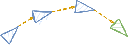
As the robot moves, it creates nodes in a graph. Constraints / edges between the nodes come from various sources — odometry estimates, scan matching, etc.

• Constraints are inherently uncertain.
• Observing previously seen areas generates constraints between non-successive poses (loop closures).

Idea of graph-based SLAM

• Use a graph to represent the problem.
• Every node is a pose of the robot during mapping.
• Every edge between two nodes is a spatial constraint between them.

Goal. Build the graph and find a node configuration that minimizes the error introduced by the constraints.

The graph

• $n$ nodes $\mathbf{x}={\mathbf{x}}_{1:n}$.
• Each ${\mathbf{x}}_i$ is a 2D or 3D transformation (the pose of the robot at time $t_i$).
• Create an edge if…
  1. The robot moves from ${\mathbf{x}}_i$ to ${\mathbf{x}}_{i+1}$ → edge corresponds to odometry.
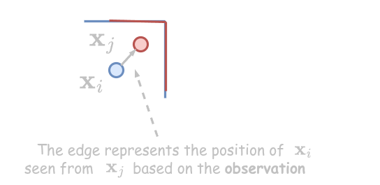
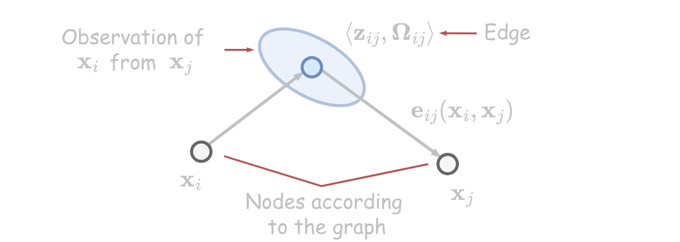
  2. The robot observes the same part of the environment from ${\mathbf{x}}_i$ and ${\mathbf{x}}_j$ → edge represents the position of ${\mathbf{x}}_j$ seen from ${\mathbf{x}}_i$ based on the observation. We construct a virtual measurement about how node $i$ sees node $j$.

Transformations

Transformations are expressed using homogeneous coordinates.

• Odometry-based edge: ${\mathbf{Z}}_{i,i+1}={\mathbf{X}}_i^{-1}{\mathbf{X}}_{i+1}$
• Observation-based edge: ${\mathbf{Z}}_{ij}={\mathbf{X}}_i^{-1}{\mathbf{X}}_j\text{(how node }i\text{ sees node }j)$

Pose graph

Goal:

$${\mathbf{x}}^{\star }=\arg \underset{\mathbf{x}}{\min }\sum _{ij}{\mathbf{e}}_{ij}^T{\mathbf{\Omega }}_{ij}{\mathbf{e}}_{ij}$$

Why this form?

Because the error term $e_{ij}$ is strongly related to the expression of a Gaussian distribution $(x-\mu {)}^T\Sigma (x-\mu )$. Minimizing ${\mathbf{e}}_{ij}^T{\mathbf{\Omega }}_{ij}{\mathbf{e}}_{ij}$ is equivalent to maximizing the likelihood of a Gaussian with mean ${\mathbf{Z}}_{ij}$ and information ${\mathbf{\Omega }}_{ij}$.

The sum across edges encodes the assumption that the constraints are independent.

The error function

For a single constraint:

$${\mathbf{e}}_{ij}({\mathbf{x}}_i,{\mathbf{x}}_j)=t2v\left({\mathbf{Z}}_{ij}^{-1}({\mathbf{X}}_i^{-1}{\mathbf{X}}_j)\right)$$

where:

• ${\mathbf{Z}}_{ij}$ is the measurement,
• ${\mathbf{X}}_i^{-1}{\mathbf{X}}_j$ is ${\mathbf{x}}_j$ referenced w.r.t. ${\mathbf{x}}_i$,
• $t2v(\cdot )$ converts a transformation matrix to a vector (e.g. $I\Rightarrow (0,0,0)$).

The error is zero iff ${\mathbf{Z}}_{ij}={\mathbf{X}}_i^{-1}{\mathbf{X}}_j$.

Gauss-Newton on the pose graph

The overall procedure mirrors the generic Gauss-Newton recipe:

• Define the error function.
• Linearize it.
• Compute its derivative.
• Set the derivative to zero.
• Solve the linear system.
• Iterate until convergence.

Linearizing the error function

Around an initial guess $\mathbf{x}$ via Taylor expansion:

$${\mathbf{e}}_{ij}(\mathbf{x}+\Delta \mathbf{x})\approx {\mathbf{e}}_{ij}(\mathbf{x})+{\mathbf{J}}_{ij}\Delta \mathbf{x},{\mathbf{J}}_{ij}=\frac{\partial {\mathbf{e}}_{ij}(\mathbf{x})}{\partial \mathbf{x}}$$

Sparsity of the Jacobian

The error ${\mathbf{e}}_{ij}(\mathbf{x})$ depends only on the two parameter blocks ${\mathbf{x}}_i$ and ${\mathbf{x}}_j$:

$${\mathbf{e}}_{ij}(\mathbf{x})={\mathbf{e}}_{ij}({\mathbf{x}}_i,{\mathbf{x}}_j)$$

The Jacobian is therefore zero everywhere except in the columns of ${\mathbf{x}}_i$ and ${\mathbf{x}}_j$.

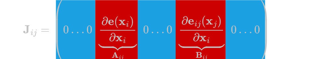
Note. This sparsity is what lets us solve the system efficiently.

Consequences of sparsity

We compute the coefficient vector $\mathbf{b}$ and matrix $\mathbf{H}$ for the system $\mathbf{H}\Delta \mathbf{x}=-\mathbf{b}$:

$${\mathbf{b}}^T=\sum _{ij}{\mathbf{e}}_{ij}^T{\mathbf{\Omega }}_{ij}{\mathbf{J}}_{ij},\mathbf{H}=\sum _{ij}{\mathbf{J}}_{ij}^T{\mathbf{\Omega }}_{ij}{\mathbf{J}}_{ij}.$$

The sparse structure of ${\mathbf{J}}_{ij}$ leads to a sparse $\mathbf{H}$ — and that sparsity pattern is exactly the adjacency matrix of the graph.

VisualizationSparsity of the H matrix

SequentialWith loop closuresPose + landmarks

# poses10

Switch between the modes to see how the H matrix block structure mirrors the graph: a sequential trajectory gives a banded tridiagonal H; loop closures add off-diagonal fill; landmarks split H into a four-block structure with a dense pose block, a sparse landmark block, and the cross-terms.

Building the linear system

For each constraint:

• Compute the error: $${\mathbf{e}}_{ij}=t2v\left({\mathbf{Z}}_{ij}^{-1}({\mathbf{X}}_i^{-1}{\mathbf{X}}_j)\right)$$
• Compute Jacobian blocks: $${\mathbf{A}}_{ij}=\frac{\partial \mathbf{e}({\mathbf{x}}_i,{\mathbf{x}}_j)}{\partial {\mathbf{x}}_i},{\mathbf{B}}_{ij}=\frac{\partial \mathbf{e}({\mathbf{x}}_i,{\mathbf{x}}_j)}{\partial {\mathbf{x}}_j}$$
• Update the coefficient vector: $${\bar{\mathbf{b}}}_i^T+={\mathbf{e}}_{ij}^T{\mathbf{\Omega }}_{ij}{\mathbf{A}}_{ij},{\bar{\mathbf{b}}}_j^T+={\mathbf{e}}_{ij}^T{\mathbf{\Omega }}_{ij}{\mathbf{B}}_{ij}$$
• Update the system matrix: $${\mathbf{H}}^{ii}+={\mathbf{A}}_{ij}^T{\mathbf{\Omega }}_{ij}{\mathbf{A}}_{ij},{\mathbf{H}}^{ij}+={\mathbf{A}}_{ij}^T{\mathbf{\Omega }}_{ij}{\mathbf{B}}_{ij},$$ $${\mathbf{H}}^{ji}+={\mathbf{B}}_{ij}^T{\mathbf{\Omega }}_{ij}{\mathbf{A}}_{ij},{\mathbf{H}}^{jj}+={\mathbf{B}}_{ij}^T{\mathbf{\Omega }}_{ij}{\mathbf{B}}_{ij}.$$

Algorithm

algorithmoptimize(x)

1. while not converged:# iterate until convergence
2. (H, b) = buildLinearSystem(x)# build sparse normal equations
3. Δx = solveSparse(H Δx = −b)# solve sparse system
4. x = x + Δx# state update
5. return x

A trivial 1D example

Three nodes and one observation per edge:

$$({\mathbf{x}}_1)\to ({\mathbf{x}}_2)\to ({\mathbf{x}}_3),z_{12}=z_{23}=1$$ $$\mathbf{x}=(0,0,0{)}^T,{\Omega }_{12}=1,{\Omega }_{23}=0.5$$

Error function: $e_{ij}=z_{ij}-(x_j-x_i)$.

1. Errors: $e_{12}=1-(0-0)=1$, $e_{23}=1-(0-0)=1$.
2. Jacobians (1×3 row vectors): $J_{12}=(1,-1,0)$, $J_{23}=(0,1,-1)$.
3. Coefficient blocks: $$b_{12}^T=e_{12}^T{\Omega }_{12}{J}_{12}=(1,-1,0),b_{23}^T=e_{23}^T{\Omega }_{23}{J}_{23}=(0,0.5,-0.5)$$ $$b^T=(1,-0.5,-0.5)$$
4. System matrix: $$H=\left(\begin{array}{ccc}1& -1& 0\\ -1& 1.5& -0.5\\ 0& -0.5& 0.5\end{array}\right)$$

Try to solve $H\Delta \mathbf{x}=-\mathbf{b}$ and you'll notice $\det (H)=0$ — $H$ is singular.

What went wrong?

• The constraints are relative between nodes.
• Any choice of poses works as long as their relative coordinates fit.
• One node needs to be fixed.

Add an extra anchor constraint to $H$:

$$H=\left(\begin{array}{ccc}2& -1& 0\\ -1& 1.5& -0.5\\ 0& -0.5& 0.5\end{array}\right)$$

This anchors $x_1$ to its position. Solving gives $\Delta x=(0,1,2{)}^T$ — exactly the configuration we'd expect.

Role of the prior

• $\mathbf{H}$ is not full rank before we fix the global reference frame.
• Fixing the global frame is strongly related to the prior $p({\mathbf{x}}_0)$.
• A Gaussian estimate about ${\mathbf{x}}_0$ adds one extra constraint.

To anchor to the origin, add an error function based on a single variable — the transformation of ${\mathbf{x}}_0$ itself:

$$\mathbf{e}({\mathbf{x}}_0)=t2v({\mathbf{X}}_0)$$

Fixing a subset of variables

When the value of certain variables during optimization is known, we may want to optimize all others and keep these fixed.

• If a variable isn't optimized, it should "disappear" from the linear system.
• Construct the full system.
• Suppress the rows and columns corresponding to the variables to fix.

Uncertainty

• $\mathbf{H}$ is the information matrix at the linearization point.
• Inverting $\mathbf{H}$ gives a (dense) covariance matrix.
• The diagonal blocks of the covariance encode the absolute uncertainties of the variables.

Relative uncertainty

To determine the relative uncertainty between two nodes ${\mathbf{x}}_i$ and ${\mathbf{x}}_j$:

• Construct $\mathbf{H}$.
• Suppress the rows / columns of ${\mathbf{x}}_i$ (this "fixes" ${\mathbf{x}}_i$).
• Compute the $j,j$ block of the inverse.
• That block contains the covariance of ${\mathbf{x}}_j$ w.r.t. the fixed ${\mathbf{x}}_i$.

VisualizationPose-graph optimization — closing the loop

⏸ Pause↺ Reset🎲 Reseed

Iter0

Noise scale1.00

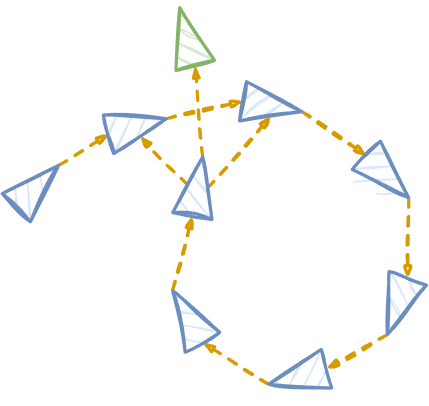
A live pose-graph optimization: the dashed circle is the ground truth, the solid coloured line is the current estimate, and the faint dashed lines are the loop-closure constraints pulling the path back together. The initial trajectory is built by integrating raw noisy odometry — it drifts off the circle. Each iteration of Gauss-Newton solves a sparse $H\Delta \mathbf{x}=-\mathbf{b}$ and pulls the estimate closer to a configuration consistent with all the relative-pose constraints.

Does all that run online?

It depends on the size of the graph. At some point the graph grows large enough that optimization becomes slower than the rate at which we add new nodes.

This leads to the hierarchical pose graph — we don't need all of the nodes to optimize our graph.

Hierarchical pose graph

Nodes can represent large chunks of nodes and be optimized as the higher-level node.

Motivation: "there's no need to optimize the whole graph when an observation is obtained."

• The front-end searches for loop closures.
• That requires comparing observations to all previously obtained ones.
• In practice we limit the search to areas where the robot is likely to be.
• This requires knowing which parts of the graph to search for data associations.

Hierarchical approach

Insight. To find loop closures, we don't need the perfect global map.

Idea. Correct only the core structure of the scene, not the overall graph. The hierarchical pose graph is a sparse approximation of the original problem.

It exploits the fact that in SLAM:

• The robot moves through the scene — it's not "teleported" to locations.
• Sensors have a limited range.

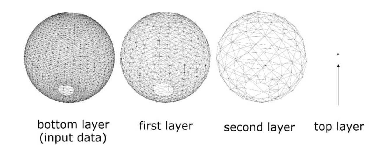
Key idea of the hierarchy

• Input is the dense graph.
• Group the nodes by local connectivity.
• For each group, select one node as a "representative".

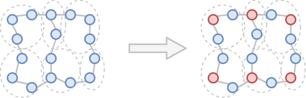
• The representatives are the nodes in a new sparsified upper-level graph.

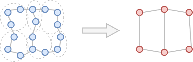
• Edges of the sparse graph are determined by the connectivity of the groups.
• The parameters of the sparse edges are estimated via local optimization.
• Process is recursive.

Only the upper level of the hierarchy is fully optimized. Changes are propagated to the lower levels only near the current robot position — the only part relevant for finding constraints.

Note. Keeping only a portion of nodes/edges makes this an approximation — but a very accurate one in practice.

Construction details

When to start a new group? A simple distance-based decision. The first node of a new group is the representative.

When to propagate information downwards? Only when there are inconsistencies.

Determining edge parameters. Given two connected groups, how do we compute a virtual observation $\mathbf{z}$ and information matrix $\mathbf{\Omega }$ for the new edge?

• Optimize the two sub-groups jointly but independently from the rest.
• The observation is the relative transformation between the two representatives.
• The information matrix comes from the diagonal block of $\mathbf{H}$: ${\mathbf{\Omega }}_{ab}=({\mathbf{H}}_{[b,b]}^{-1}{)}^{-1}$

Effectively we fix ${\mathbf{x}}_a$, compute ${\mathbf{x}}_b$ relative to it, invert $\mathbf{H}$, cut out the $[b,b]$ block, and invert it back.

Propagating information downwards

All representatives are nodes from the lower level. Information is propagated downwards by transforming the group at the lower level using a rigid-body transformation. Only if the lower level becomes inconsistent do we optimize it.

For the best possible map

• Run the optimization on the lowest level at the end.
• For offline processing with all constraints, the hierarchy helps convergence faster in the presence of large errors.
• In that case, one pass up the tree (to construct the edges) followed by one pass down is sufficient.

Consistency check

How well does the top level represent the original input? Compute the probability mass of the marginal distribution in the highest level vs the true estimated (original problem, lowest level).

Conclusions

• The back-end of the SLAM problem can be effectively solved with Gauss-Newton.
• The $\mathbf{H}$ matrix is typically sparse.
• This sparsity allows for efficient solution of the linear system.
• One of the state-of-the-art solutions for computing maps.
• Hierarchical pose graphs enable approximate online solutions.

---

Reading material

Least-squares SLAM

• Grisetti et al. A Tutorial on Graph-based SLAM, 2010.

Hierarchical approach

• Grisetti et al. Hierarchical Optimization on Manifolds for Online 2D and 3D Mapping, 2010.