Motion & Sensor Models

Below we detail common motion and observation models used in SLAM, with small Python implementations.

Motion models

In robotics, the motion model describes how the robot state evolves from one time step to the next given a previous state and a control input. Formally, it is the posterior:

Real-world motion always involves inherent uncertainty, so we explicitly model it. Two common motion models in practice:

1. Odometry-based motion model (typically wheeled robots).
2. Velocity-based motion model (often aerial or legged robots).

1. Odometry-based motion model

The odometry model relies on wheel encoders that count wheel rotations to estimate displacement. Tyre pressure, slip, or uneven terrain introduce drift over time — odometry measurements inherently contain uncertainty.

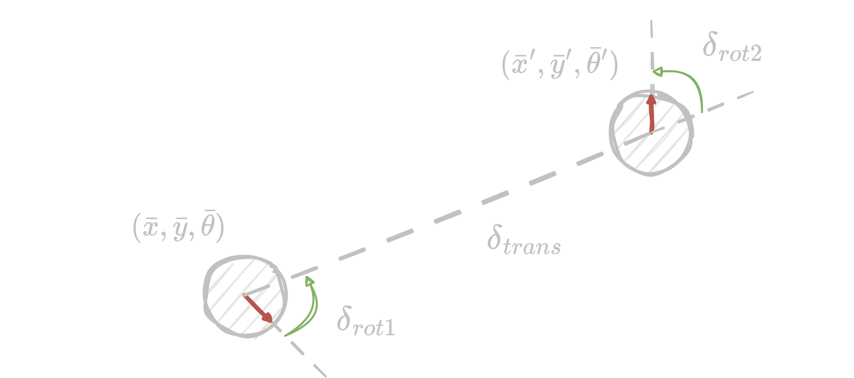
Odometry measurements. Given the previous robot pose $(\bar{x},\bar{y},\bar{\theta })$ and the new pose $({\bar{x}}^{\prime },{\bar{y}}^{\prime },{\bar{\theta }}^{\prime })$, define the odometry measurement $u$ as a triple of rotation/translation changes:

Each component:

• Translational displacement: $${\delta }_{trans}=\sqrt{({\bar{x}}^{\prime }-\bar{x}{)}^2+({\bar{y}}^{\prime }-\bar{y}{)}^2}$$
• Initial rotation (to face the direction of motion): $${\delta }_{rot1}=atan2({\bar{y}}^{\prime }-\bar{y},{\bar{x}}^{\prime }-\bar{x})-\bar{\theta }$$
• Final rotation (to reach the final orientation): $${\delta }_{rot2}={\bar{\theta }}^{\prime }-\bar{\theta }-{\delta }_{rot1}$$

So the motion is decomposed into three sequential steps:

1. Initial rotation (${\delta }_{rot1}$) aligning the robot toward the target position.
2. Translational motion (${\delta }_{trans}$) moving the robot forward.
3. Final rotation (${\delta }_{rot2}$) aligning the robot with the desired orientation.

Modelling uncertainty. Noise in each measurement is typically modelled as additive Gaussian:

where $\Sigma$ is the covariance matrix.

Python example — odometry motion model

import numpy as np
 
def motion_model_odometry(u, x_prev, noise_std=(0, 0, 0)):
    """
    Sample-based odometry motion model.
    u        : (delta_rot1, delta_trans, delta_rot2)
    x_prev   : (x, y, theta)
    noise_std: per-component Gaussian std
    """
    d_rot1, d_trans, d_rot2 = u
 
    d_rot1_hat  = d_rot1  + np.random.normal(0, noise_std[0])
    d_trans_hat = d_trans + np.random.normal(0, noise_std[1])
    d_rot2_hat  = d_rot2  + np.random.normal(0, noise_std[2])
 
    x     = x_prev[0] + d_trans_hat * np.cos(x_prev[2] + d_rot1_hat)
    y     = x_prev[1] + d_trans_hat * np.sin(x_prev[2] + d_rot1_hat)
    theta = x_prev[2] + d_rot1_hat + d_rot2_hat
 
    return np.array([x, y, theta])

Driving an initial pose through a list of commands yields two trajectories — one without noise (ideal ground truth) and one with Gaussian noise (realistic conditions). Plotting both side-by-side shows how small per-step errors accumulate into a large drift.

The ground-truth path (green) is what we commanded; each thin teal line is one stochastic realization of the same command sequence under per-step Gaussian noise. The cloud of endpoints widens dramatically with the number of steps — this is dead-reckoning drift, and it is exactly why we need observations to correct the pose.

2. Velocity-based motion model

A velocity-based motion model is expressed through two velocities: a translational velocity $v$ and a rotational velocity $w$. This results in arc-like trajectories.

Given current state $(x,y,\theta )$ and control $u=(v,w{)}^T$, the updated state after $\Delta t$ is:

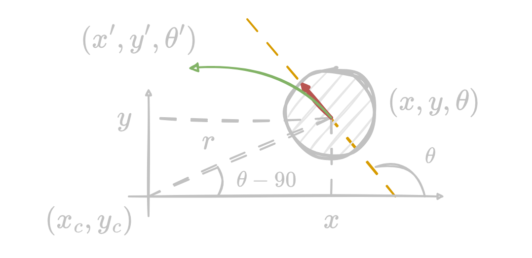
Note. Arc-like motion alone does not allow specifying a particular final orientation, so we add an extra term $\gamma \Delta t$ to adjust orientation explicitly.

Python example — velocity motion model

def motion_model_velocity(u, x_prev, dt=1.0, noise_std=(0, 0, 0)):
    """
    Sample-based velocity motion model.
    u        : (v, w, gamma)
    x_prev   : (x, y, theta)
    """
    v, w, gamma = u
    v_hat     = v     + np.random.normal(0, noise_std[0])
    w_hat     = w     + np.random.normal(0, noise_std[1])
    gamma_hat = gamma + np.random.normal(0, noise_std[2])
 
    if abs(w_hat) > 1e-6:
        x_new = x_prev[0] - (v_hat/w_hat) * np.sin(x_prev[2]) \
                          + (v_hat/w_hat) * np.sin(x_prev[2] + w_hat*dt)
        y_new = x_prev[1] + (v_hat/w_hat) * np.cos(x_prev[2]) \
                          - (v_hat/w_hat) * np.cos(x_prev[2] + w_hat*dt)
    else:
        # Straight line when w == 0
        x_new = x_prev[0] + v_hat * dt * np.cos(x_prev[2])
        y_new = x_prev[1] + v_hat * dt * np.sin(x_prev[2])
    theta_new = x_prev[2] + w_hat * dt + gamma_hat * dt
 
    return np.array([x_new, y_new, theta_new])

Sampling 1000 trajectories with noise on $v$ only, $w$ only, and both together makes the directional structure of the uncertainty very visible: $v$-noise spreads the cloud along the heading, $w$-noise smears it perpendicular to the heading, and combined noise yields a tilted "banana" shape.

Conclusion

A key takeaway from these examples: the motion we command is not the motion we get. Real actuators have slip, drift, and quantization. That's why every Bayesian filter for robot state estimation treats motion probabilistically.

Observation (sensor) models

An observation model relates the robot's state to sensor measurements. It is the likelihood of getting measurement $z_t$ given state $x_t$:

Sensor measurements contain noise, so the model must explicitly account for it.

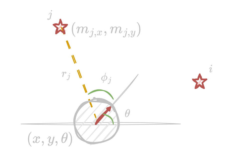
Range-bearing sensor model (landmark-based)

A typical 2D LiDAR or radar measures landmarks by providing:

• Range — distance from the robot to the landmark.
• Bearing — angle from the robot's orientation to the landmark.

Given the robot state $x_t=[x,y,\theta {]}^T$ and a landmark $m_j=[m_{j,x},m_{j,y}{]}^T$, the observation $z_t^j$ is:

where:

• $r_j$ is the range,
• ${\phi }_j$ is the bearing,
• $q\sim \mathcal{N}(0,Q)$ is the measurement noise, with

Python example — range-bearing observation

def range_bearing_observation(x, landmark, noise_std=(0, 0)):
    """
    2D range-bearing sensor model with Gaussian noise.
    x        : (x, y, theta)
    landmark : (lx, ly)
    """
    dx = landmark[0] - x[0]
    dy = landmark[1] - x[1]
 
    r   = np.sqrt(dx**2 + dy**2)
    phi = np.arctan2(dy, dx) - x[2]
 
    r_noisy   = r   + np.random.normal(0, noise_std[0])
    phi_noisy = phi + np.random.normal(0, noise_std[1])
 
    return np.array([r_noisy, phi_noisy])

Each tick re-samples the measurement noise, so the noisy rays (teal) dance around the true bearing (dashed). As you crank up ${\sigma }_r$ or ${\sigma }_{\phi }$ the landmark endpoints scatter farther — this scatter pattern is exactly what the filter's measurement-noise covariance $Q$ has to model.

Interactive demos in the notebooks

The original notebook includes three interactive pygame demonstrations that run locally:

• Interactive odometry motion model — drive a robot with arrow keys and watch the noisy trajectory drift away from the ground-truth pose.
• Interactive observation model — a rotating sensor beam on a floor-plan image; landmarks appear on the right panel as the beam registers noisy hits.
• Combined motion + observation — both effects together: the noisy trajectory and the projected landmarks accumulate map-drift over time.

These visualizations are best run from the source repository — see the original notebook for the full Pygame implementation. The intuition they build is the central motivation for filtering:

Noisy motion and noisy observations make the map and the pose drift. We need a probabilistic filter — Kalman, EKF, particle filter — to predict the state and correct it from observations.

Reading material

On motion and observation models

• Thrun, Burgard, Fox. Probabilistic Robotics, Chapters 5 & 6.