Landmark Graph-based SLAM

Recap

• Use a graph to represent the SLAM problem.
• Every node in the graph corresponds to a pose of the robot during mapping.
• Every edge between two nodes is a spatial constraint between them.

Graph-based SLAM: build the graph and find a node configuration that minimizes the error introduced by the constraints.

The graph

So far:

• Vertices: robot poses $(x,y,\theta )$.
• Edges: virtual observations (transformations) between robot poses.

This lesson's topic: how to deal with landmarks?

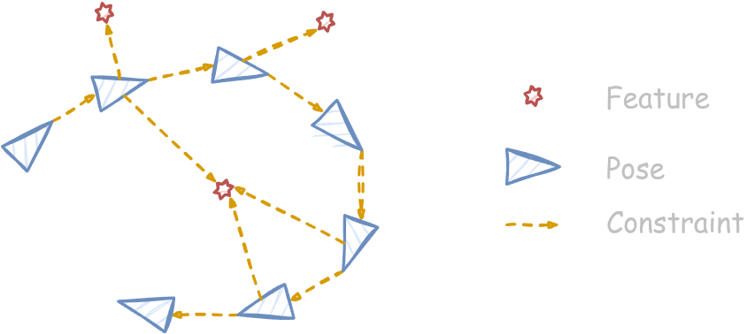
The graph with landmarks

Nodes can now represent:

• Robot poses,
• Landmark locations.

Edges can represent:

• Landmark observations,
• Odometry measurements.

The minimization now optimizes both the landmark locations and the robot poses.

2D landmarks

A landmark is a $(x,y)$ point in the world. A relative observation is also in $(x,y)$.

Landmark observation

Expected observation (using an $(x,y)$ sensor):

• ${\mathbf{R}}_i$ — rotation matrix of robot pose $i$.
• ${\mathbf{t}}_i$ — robot translation.
• ${\mathbf{x}}_j$ — landmark position.

Error function:

Bearing-only observations

In many real-world scenarios, sensors don't provide range information — only bearing (direction) of a feature relative to the robot:

• Cameras — a visual feature can be detected in the image plane, but its actual distance is unknown without additional geometric reasoning or motion.
• Directional antennas — measure direction to a source but not range.
• Monocular SLAM — a single camera setup can only estimate bearing; depth is inferred gradually through motion (triangulation).

The robot observes only the bearing toward the landmark, but the landmark itself is still a 2D point.

Expected observation with a bearing-only sensor:

Error function:

Where is the robot?

If the robot observes one $(x,y)$ landmark, the robot can be anywhere on a circle around the landmark — a 1D solution space, constrained by distance and orientation.

How many 2D landmark observations are needed to fully resolve the pose? → At least two.

If the robot observes one landmark bearing-only, the robot can be anywhere in the XY-plane — a 2D solution space, constrained by the robot's orientation.

How many bearing-only observations are needed to resolve a pose? → At least three.

The rank of the matrix $\mathbf{H}$

In landmark-based SLAM, the system can be under-determined:

• The rank of $\mathbf{H}$ is less than or equal to the sum of the ranks of its constraints.
• To determine a unique solution, $\mathbf{H}$ must have full rank.

Under-determined systems

There's no guarantee of a full-rank system:

• Landmarks may be observed only once.
• The robot might lack odometry.

We handle these cases by adding a damping factor to $\mathbf{H}$. Instead of solving $\mathbf{H}\Delta \mathbf{x}=-\mathbf{b}$, we solve

Effect of the damping factor $\lambda$:

• Makes the system positive definite.
• Acts as a weighted combination of Gauss-Newton and steepest descent → Levenberg-Marquardt.
• Stabilizes convergence and avoids large steps.

Switch to Pose + landmarks to see the four-block H structure used by landmark-based graph SLAM: a dense block for the pose-pose part (top-left), a sparse near-diagonal block for the landmark-landmark part (bottom-right), and the cross-blocks linking poses to the landmarks they observed. This block sparsity is what makes the Schur complement trick so effective in bundle adjustment — eliminate the landmark block, solve for poses, then back-substitute.

A working example: 2D pose-landmark graph with Levenberg-Marquardt

The notebook walks through a full 2D pose-landmark SLAM example: noisy odometry, loop closures, and range-bearing landmark observations are folded into a single non-linear least-squares problem solved with Levenberg-Marquardt.

The pipeline is:

1. Synthetic world (clean reference). Sample $N$ poses on a circle (closed loop, first pose at the origin) and scatter $M$ landmarks around the trajectory.
2. Graph construction.
   • Odometry edges connect $i\to i+1$ with a relative motion $z_{ij}$ in the local frame.
   • Loop-closure edges connect $i\to i+10$ to inject long-baseline constraints and reduce drift; add $(N-1)\to 0$ to close the loop.
   • Landmark edges connect pose $i$ to landmark $\ell$ with a range-bearing measurement $z_{i\ell }=[r,\varphi {]}^T$ for visible landmarks (within max range / FOV).
3. Measurement noise. Perturb odometry with Gaussian noise in translation/rotation and landmark measurements with Gaussian noise in range/bearing. The optimizer sees only these noisy factors.
4. Initial guess.
   • Poses: integrate noisy odometry forward from node 0; accumulates drift around the loop.
   • Landmarks: back-project the first observation of each landmark from the current pose estimate.
5. Levenberg-Marquardt optimization.
   • Residuals:
     • Pose-pose: $e_{ij}=\mathrm{rel}(x_i,x_j)\ominus z_{ij}$ with angle wrapping.
     • Pose-landmark: $e_{i\ell }=\left[\begin{array}{c}\hat{r}-r\\ \mathrm{wrap}(\hat{\varphi }-\varphi )\end{array}\right]$, with $\hat{r},\hat{\varphi }$ from the current $x_i,m_{\ell }$.
   • Linearization: form analytic Jacobians $J$ for both factor types and accumulate the normal equations $H=\sum J^T\Omega J,b=\sum J^T\Omega e$.
   • Gauge fixing: add a strong prior on pose 0 (position and yaw) to define a reference frame.
   • LM damping: solve $(H+\lambda \mathrm{diag}(H))\Delta =-b$. If the trial decreases the total cost, accept and reduce $\lambda$; otherwise reject and increase $\lambda$. Iterate until convergence.

import numpy as np
 
def wrap(a):
    return (a + np.pi) % (2 * np.pi) - np.pi
 
def R2(theta):
    c, s = np.cos(theta), np.sin(theta)
    return np.array([[c, -s], [s, c]])
 
def relative_pose(xi, xj):
    """Predicted odometry z_ij from poses xi -> xj (both 3-vectors)."""
    RiT = R2(xi[2]).T
    dt  = RiT @ (xj[:2] - xi[:2])
    dth = wrap(xj[2] - xi[2])
    return np.array([dt[0], dt[1], dth])

The full implementation — including Jacobians for both factor types, the LM accept/reject loop, gauge fixing via a strong prior on pose 0, and the convergence plots — is in notebooks/3_graph_based/3_landmark_graph_slam.ipynb.

Bundle adjustment

Bundle adjustment is the classical least-squares problem from computer vision. It jointly optimizes camera poses (extrinsics), sometimes intrinsics, and 3D point positions so that projected points best match observed image features.

• 3D reconstruction from images taken from different viewpoints.
• Minimizes the reprojection error.
• Typically solved with Levenberg-Marquardt.
• Developed in photogrammetry during the 1950s.

The structure is identical to landmark-based graph SLAM: poses + landmark (3D point) variables, with sparse cross-blocks linking the pose a landmark was seen from to the landmark itself. The Schur complement is the standard trick to factor out the landmark block efficiently.

Summary

• Graph-based SLAM extended to handle landmarks as graph nodes.
• The rank of $\mathbf{H}$ matters — under-determined systems need extra constraints or damping.
• Levenberg-Marquardt is the workhorse optimizer: trust-region damping plus accept/reject step control gives a robust algorithm.
• Bundle adjustment is structurally the same problem; sparsity keeps it tractable at scale.